Steps to follow in any data processing:

1. Know the problem
2. Obtain the training and test data
3. Preprocessing and data cleaning
4. Exploratory analysis
5. Develop a model
6. Visualize and report the solution and results.

Data collection

# data analysis and wrangling
import pandas as pd
import numpy as np
import random as rnd

# visualization
import seaborn as sns
import matplotlib.pyplot as plt
%matplotlib inline

# machine learning
from sklearn.linear_model import LogisticRegression
from sklearn.svm import SVC, LinearSVC
from sklearn.ensemble import RandomForestClassifier
from sklearn.neighbors import KNeighborsClassifier
from sklearn.naive_bayes import GaussianNB
from sklearn.linear_model import Perceptron
from sklearn.linear_model import SGDClassifier
from sklearn.tree import DecisionTreeClassifier

train = pd.read_csv("train.csv")
test = pd.read_csv("test.csv")

#dataframes array
combine = [train, test] 

pd.set_option('display.expand_frame_repr', False)

combine

[     PassengerId  Survived  Pclass                                               Name     Sex   Age  SibSp  Parch            Ticket     Fare Cabin Embarked
 0              1         0       3                            Braund, Mr. Owen Harris    male  22.0      1      0         A/5 21171   7.2500   NaN        S
 1              2         1       1  Cumings, Mrs. John Bradley (Florence Briggs Th...  female  38.0      1      0          PC 17599  71.2833   C85        C
 2              3         1       3                             Heikkinen, Miss. Laina  female  26.0      0      0  STON/O2. 3101282   7.9250   NaN        S
 3              4         1       1       Futrelle, Mrs. Jacques Heath (Lily May Peel)  female  35.0      1      0            113803  53.1000  C123        S
 4              5         0       3                           Allen, Mr. William Henry    male  35.0      0      0            373450   8.0500   NaN        S
 ..           ...       ...     ...                                                ...     ...   ...    ...    ...               ...      ...   ...      ...
 886          887         0       2                              Montvila, Rev. Juozas    male  27.0      0      0            211536  13.0000   NaN        S
 887          888         1       1                       Graham, Miss. Margaret Edith  female  19.0      0      0            112053  30.0000   B42        S
 888          889         0       3           Johnston, Miss. Catherine Helen "Carrie"  female   NaN      1      2        W./C. 6607  23.4500   NaN        S
 889          890         1       1                              Behr, Mr. Karl Howell    male  26.0      0      0            111369  30.0000  C148        C
 890          891         0       3                                Dooley, Mr. Patrick    male  32.0      0      0            370376   7.7500   NaN        Q
 
 [891 rows x 12 columns],
      PassengerId  Pclass                                          Name     Sex   Age  SibSp  Parch              Ticket      Fare Cabin Embarked
 0            892       3                              Kelly, Mr. James    male  34.5      0      0              330911    7.8292   NaN        Q
 1            893       3              Wilkes, Mrs. James (Ellen Needs)  female  47.0      1      0              363272    7.0000   NaN        S
 2            894       2                     Myles, Mr. Thomas Francis    male  62.0      0      0              240276    9.6875   NaN        Q
 3            895       3                              Wirz, Mr. Albert    male  27.0      0      0              315154    8.6625   NaN        S
 4            896       3  Hirvonen, Mrs. Alexander (Helga E Lindqvist)  female  22.0      1      1             3101298   12.2875   NaN        S
 ..           ...     ...                                           ...     ...   ...    ...    ...                 ...       ...   ...      ...
 413         1305       3                            Spector, Mr. Woolf    male   NaN      0      0           A.5. 3236    8.0500   NaN        S
 414         1306       1                  Oliva y Ocana, Dona. Fermina  female  39.0      0      0            PC 17758  108.9000  C105        C
 415         1307       3                  Saether, Mr. Simon Sivertsen    male  38.5      0      0  SOTON/O.Q. 3101262    7.2500   NaN        S
 416         1308       3                           Ware, Mr. Frederick    male   NaN      0      0              359309    8.0500   NaN        S
 417         1309       3                      Peter, Master. Michael J    male   NaN      1      1                2668   22.3583   NaN        C
 
 [418 rows x 11 columns]]

Exploratory analysis

Features description

print(train.columns.values)

['PassengerId' 'Survived' 'Pclass' 'Name' 'Sex' 'Age' 'SibSp' 'Parch'
 'Ticket' 'Fare' 'Cabin' 'Embarked']

print(test.columns.values)

['PassengerId' 'Pclass' 'Name' 'Sex' 'Age' 'SibSp' 'Parch' 'Ticket' 'Fare'
 'Cabin' 'Embarked']

print(train.info())
print('-'*40)
print(test.info())

<class 'pandas.core.frame.DataFrame'>
RangeIndex: 891 entries, 0 to 890
Data columns (total 12 columns):
 #   Column       Non-Null Count  Dtype  
---  ------       --------------  -----  
 0   PassengerId  891 non-null    int64  
 1   Survived     891 non-null    int64  
 2   Pclass       891 non-null    int64  
 3   Name         891 non-null    object 
 4   Sex          891 non-null    object 
 5   Age          714 non-null    float64
 6   SibSp        891 non-null    int64  
 7   Parch        891 non-null    int64  
 8   Ticket       891 non-null    object 
 9   Fare         891 non-null    float64
 10  Cabin        204 non-null    object 
 11  Embarked     889 non-null    object 
dtypes: float64(2), int64(5), object(5)
memory usage: 83.7+ KB
None
----------------------------------------
<class 'pandas.core.frame.DataFrame'>
RangeIndex: 418 entries, 0 to 417
Data columns (total 11 columns):
 #   Column       Non-Null Count  Dtype  
---  ------       --------------  -----  
 0   PassengerId  418 non-null    int64  
 1   Pclass       418 non-null    int64  
 2   Name         418 non-null    object 
 3   Sex          418 non-null    object 
 4   Age          332 non-null    float64
 5   SibSp        418 non-null    int64  
 6   Parch        418 non-null    int64  
 7   Ticket       418 non-null    object 
 8   Fare         417 non-null    float64
 9   Cabin        91 non-null     object 
 10  Embarked     418 non-null    object 
dtypes: float64(2), int64(4), object(5)
memory usage: 36.0+ KB
None

Categorical variable: defines a category –> Male,Female,Undefined –> can be 0 - 1 … or with words

Ordinal variable: defines a sorted category –> dirty, medium, clean

Numerical variable –> discrete or continuous

• Discrete numerical variable: counted items –> number of children
• Continuous numerical variable: measurable characteristics –> weight

---

print(train['Survived'])

0      0
1      1
2      1
3      1
4      0
      ..
886    0
887    1
888    0
889    1
890    0
Name: Survived, Length: 891, dtype: int64

Categorical features: Survived, Sex, Embarked

Ordinal features: Pclass

Discrete numerical features: PassengerID, SibSp, Parch

Continuous numerical features: Age, Fare

Mixed features: Ticket, Cabin

Error-prone features: Name

Attributes with null values require correction.

In the training data, Age Cabin Embarked has null values.

In the test data, Age Cabin has null values.

train.describe(include='all') 

	PassengerId	Survived	Pclass	Name	Sex	Age	SibSp	Parch	Ticket	Fare	Cabin	Embarked
count	891.000000	891.000000	891.000000	891	891	714.000000	891.000000	891.000000	891	891.000000	204	889
unique	NaN	NaN	NaN	891	2	NaN	NaN	NaN	681	NaN	147	3
top	NaN	NaN	NaN	Seward, Mr. Frederic Kimber	male	NaN	NaN	NaN	CA. 2343	NaN	B96 B98	S
freq	NaN	NaN	NaN	1	577	NaN	NaN	NaN	7	NaN	4	644
mean	446.000000	0.383838	2.308642	NaN	NaN	29.699118	0.523008	0.381594	NaN	32.204208	NaN	NaN
std	257.353842	0.486592	0.836071	NaN	NaN	14.526497	1.102743	0.806057	NaN	49.693429	NaN	NaN
min	1.000000	0.000000	1.000000	NaN	NaN	0.420000	0.000000	0.000000	NaN	0.000000	NaN	NaN
25%	223.500000	0.000000	2.000000	NaN	NaN	20.125000	0.000000	0.000000	NaN	7.910400	NaN	NaN
50%	446.000000	0.000000	3.000000	NaN	NaN	28.000000	0.000000	0.000000	NaN	14.454200	NaN	NaN
75%	668.500000	1.000000	3.000000	NaN	NaN	38.000000	1.000000	0.000000	NaN	31.000000	NaN	NaN
max	891.000000	1.000000	3.000000	NaN	NaN	80.000000	8.000000	6.000000	NaN	512.329200	NaN	NaN

train.hist('Survived')

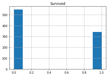
There is not too much imbalance between classes.

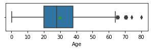
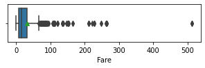
valores = ['Age','Fare']
for col in valores:
    fig,ax = plt.subplots(1,1,figsize=(5,1))    
    sns.boxplot(x=train[col],showmeans=True)
    plt.show()

Correlation analysis between variables.

We do it with features that do not have any null value and that are categorical (Sex), ordinal (Pclass) or discrete numerical (SibSp,Parch).

train[['Pclass','Survived']].groupby(['Pclass'],as_index=False).mean().sort_values(by='Survived',ascending=False)

	Pclass	Survived
0	1	0.629630
1	2	0.472826
2	3	0.242363

train[['Sex','Survived']].groupby(['Sex'],as_index=False).mean().sort_values(by='Survived',ascending=False)

	Sex	Survived
0	female	0.742038
1	male	0.188908

train[['SibSp','Survived']].groupby(['SibSp'],as_index=False).mean().sort_values(by='Survived',ascending=False)

	SibSp	Survived
1	1	0.535885
2	2	0.464286
0	0	0.345395
3	3	0.250000
4	4	0.166667
5	5	0.000000
6	8	0.000000

train[['Parch','Survived']].groupby(['Parch'],as_index=False).mean().sort_values(by='Survived',ascending=False)

	Parch	Survived
3	3	0.600000
1	1	0.550847
2	2	0.500000
0	0	0.343658
5	5	0.200000
4	4	0.000000
6	6	0.000000

Data visualization analysis

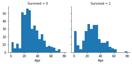
Correlation between numerical variables and our Survived solution

Histogram -> continuous numerical variables

g = sns.FacetGrid(train, col='Survived')

g.map(plt.hist, 'Age', bins=20)

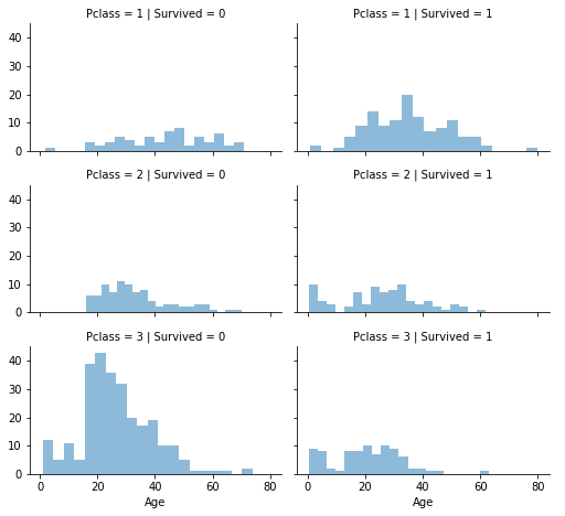
Correlation with numerical and ordinal features

grid = sns.FacetGrid(train, col='Survived', row='Pclass', height=2.2, aspect=1.6)
grid.map(plt.hist, 'Age', alpha=0.5, bins=20)
grid.add_legend()

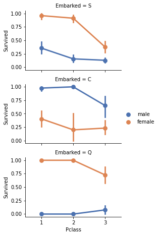
Correlation of categorical variables

grid = sns.FacetGrid(train, row='Embarked', height=2.2, aspect=1.6)
grid.map(sns.pointplot, 'Pclass','Survived','Sex', palette='deep')
grid.add_legend()

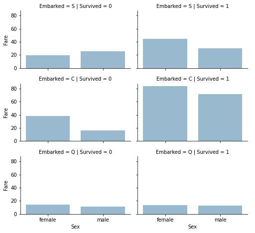
Correlation between categorical and numerical variables.

grid = sns.FacetGrid(train, row='Embarked', col='Survived', height=2.2, aspect=1.6)
grid.map(sns.barplot, 'Sex', 'Fare', alpha=0.5, ci=None)
grid.add_legend()

DATA PREPARING

Dropping features

train = train.drop(['Ticket', 'Cabin'], axis=1)
test = test.drop(['Ticket', 'Cabin'], axis=1)

combine = [train,test]
print(combine[0].shape)
print(combine[1].shape)

(891, 10)
(418, 9)

Feature extracting

for dataset in combine:
  dataset['Title'] = dataset.Name.str.extract('([A-Za-z]+)\.', expand=False)

pd.crosstab(train['Title'], train['Sex'])

Sex	female	male
Title
Capt	0	1
Col	0	2
Countess	1	0
Don	0	1
Dr	1	6
Jonkheer	0	1
Lady	1	0
Major	0	2
Master	0	40
Miss	182	0
Mlle	2	0
Mme	1	0
Mr	0	517
Mrs	125	0
Ms	1	0
Rev	0	6
Sir	0	1

for dataset in combine:
  dataset['Title'] = dataset['Title'].replace(['Lady', 'Countess', 'Capt', 'Col', 'Don',\
                                               'Dr', 'Major', 'Rev','Sir','Jonkheer','Dona'], 'Rare')
  dataset['Title'] = dataset['Title'].replace(['Mlle','Ms'],'Miss')
  dataset['Title'] = dataset['Title'].replace('Mme','Mrs')

train[['Title','Survived']].groupby(['Title'],as_index=False).mean()

	Title	Survived
0	Master	0.575000
1	Miss	0.702703
2	Mr	0.156673
3	Mrs	0.793651
4	Rare	0.347826

titles = {"Mr":1,"Miss":2,"Mrs":3,"Master":4,"Rare":5}

for dataset in combine:
  dataset['Title']= dataset['Title'].map(titles)
  dataset['Title']= dataset['Title'].fillna(0)

train.head()

	PassengerId	Survived	Pclass	Name	Sex	Age	SibSp	Parch	Fare	Embarked	Title
0	1	0	3	Braund, Mr. Owen Harris	male	22.0	1	0	7.2500	S	1
1	2	1	1	Cumings, Mrs. John Bradley (Florence Briggs Th...	female	38.0	1	0	71.2833	C	3
2	3	1	3	Heikkinen, Miss. Laina	female	26.0	0	0	7.9250	S	2
3	4	1	1	Futrelle, Mrs. Jacques Heath (Lily May Peel)	female	35.0	1	0	53.1000	S	3
4	5	0	3	Allen, Mr. William Henry	male	35.0	0	0	8.0500	S	1

train = train.drop(['Name', 'PassengerId'], axis=1)
test = test.drop('Name', axis=1) 
combine = [train,test]
print(train.shape,test.shape)

(891, 9) (418, 9)

test.head()

	PassengerId	Pclass	Sex	Age	SibSp	Parch	Fare	Embarked	Title
0	892	3	male	34.5	0	0	7.8292	Q	1
1	893	3	female	47.0	1	0	7.0000	S	3
2	894	2	male	62.0	0	0	9.6875	Q	1
3	895	3	male	27.0	0	0	8.6625	S	1
4	896	3	female	22.0	1	1	12.2875	S	3

Convert categorical feature

Strings –> Numerical values

for dataset in combine:
  dataset['Sex']= dataset['Sex'].map({'female':1, 'male':0}).astype(int)

train.head()

	Survived	Pclass	Sex	Age	SibSp	Parch	Fare	Embarked	Title
0	0	3	0	22.0	1	0	7.2500	S	1
1	1	1	1	38.0	1	0	71.2833	C	3
2	1	3	1	26.0	0	0	7.9250	S	2
3	1	1	1	35.0	1	0	53.1000	S	3
4	0	3	0	35.0	0	0	8.0500	S	1

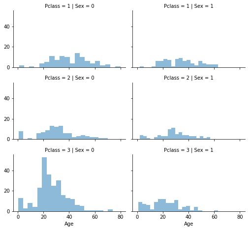
Completing a numerical continuous feature

grid = sns.FacetGrid(train, row='Pclass', col='Sex', height=2.2, aspect=1.6)
grid.map(plt.hist,'Age',alpha=.5,bins=20)
grid.add_legend()

guess_ages = np.zeros((2,3))
guess_ages

array([[0., 0., 0.],
       [0., 0., 0.]])

for dataset in combine:
  for i in range(0,2):
    for j in range(0,3):
      #print(dataset[(dataset['Sex']==i) & (dataset['Pclass']==j+1)]['Age']) 
      guess_df = dataset[(dataset['Sex']==i) & (dataset['Pclass']==j+1)]['Age'].dropna() 
      #print(guess_df) 
      age_guess = guess_df.median()
      guess_ages[i,j]=int (age_guess/0.5+0.5)*0.5
  
  for i in range(0, 2):
        for j in range(0, 3):
            dataset.loc[ (dataset.Age.isnull()) & (dataset.Sex == i) & (dataset.Pclass == j+1),'Age'] = guess_ages[i,j]
        
  dataset['Age'] = dataset['Age'].astype(int)

train.head()

	Survived	Pclass	Sex	Age	SibSp	Parch	Fare	Embarked	Title
0	0	3	0	22	1	0	7.2500	S	1
1	1	1	1	38	1	0	71.2833	C	3
2	1	3	1	26	0	0	7.9250	S	2
3	1	1	1	35	1	0	53.1000	S	3
4	0	3	0	35	0	0	8.0500	S	1

train['AgeBand'] = pd.cut(train['Age'],5)
train[['AgeBand','Survived']].groupby(['AgeBand'],as_index=False).mean().sort_values(by='AgeBand',ascending=True)

	AgeBand	Survived
0	(-0.08, 16.0]	0.550000
1	(16.0, 32.0]	0.337374
2	(32.0, 48.0]	0.412037
3	(48.0, 64.0]	0.434783
4	(64.0, 80.0]	0.090909

for dataset in combine:
  dataset.loc[dataset['Age']<=16,'Age']=0
  dataset.loc[(dataset['Age']>16) & (dataset['Age']<=32),'Age']=1
  dataset.loc[(dataset['Age']>32) & (dataset['Age']<=48),'Age']=2
  dataset.loc[(dataset['Age']>48) & (dataset['Age']<=64),'Age']=3
  dataset.loc[dataset['Age']>64,'Age']=4

train.head()

	Survived	Pclass	Sex	Age	SibSp	Parch	Fare	Embarked	Title	AgeBand
0	0	3	0	1	1	0	7.2500	S	1	(16.0, 32.0]
1	1	1	1	2	1	0	71.2833	C	3	(32.0, 48.0]
2	1	3	1	1	0	0	7.9250	S	2	(16.0, 32.0]
3	1	1	1	2	1	0	53.1000	S	3	(32.0, 48.0]
4	0	3	0	2	0	0	8.0500	S	1	(32.0, 48.0]

train = train.drop(['AgeBand'],axis=1)
combine = [train,test]

for dataset in combine:
  dataset['FamilySize'] = dataset['Parch'] + dataset['SibSp'] + 1

train[['FamilySize','Survived']].groupby(['FamilySize'],as_index=False).mean().sort_values(by='Survived',ascending=False)

	FamilySize	Survived
3	4	0.724138
2	3	0.578431
1	2	0.552795
6	7	0.333333
0	1	0.303538
4	5	0.200000
5	6	0.136364
7	8	0.000000
8	11	0.000000

for dataset in combine:
  dataset['IsAlone']=0
  dataset.loc[dataset['FamilySize']==1, 'IsAlone'] = 1 

train[['IsAlone','Survived']].groupby(['IsAlone'],as_index=False).mean()

	IsAlone	Survived
0	0	0.505650
1	1	0.303538

train = train.drop(['Parch','SibSp','FamilySize'],axis=1)
test = test.drop(['Parch','SibSp','FamilySize'],axis=1)
combine=[train,test]

train.head()

	Survived	Pclass	Sex	Age	Fare	Embarked	Title	IsAlone
0	0	3	0	1	7.2500	S	1	0
1	1	1	1	2	71.2833	C	3	0
2	1	3	1	1	7.9250	S	2	1
3	1	1	1	2	53.1000	S	3	0
4	0	3	0	2	8.0500	S	1	1

for dataset in combine:
  dataset['Age*Class'] = dataset.Age * dataset.Pclass

train.loc[:,['Age*Class','Age','Pclass']].head(10)

	Age*Class	Age	Pclass
0	3	1	3
1	2	2	1
2	3	1	3
3	2	2	1
4	6	2	3
5	3	1	3
6	3	3	1
7	0	0	3
8	3	1	3
9	0	0	2

train[['Age*Class','Survived']].groupby('Age*Class',as_index=False).mean()

	Age*Class	Survived
0	0	0.550000
1	1	0.728814
2	2	0.520408
3	3	0.277487
4	4	0.415094
5	6	0.149425
6	8	0.000000
7	9	0.111111
8	12	0.000000

Completing a categorical feature

freq_port = train['Embarked'].dropna().mode()[0]
freq_port

'S'

for dataset in combine:
  dataset['Embarked'] = dataset['Embarked'].fillna(freq_port)

train[['Embarked','Survived']].groupby('Embarked',as_index=False).mean().sort_values(by='Survived',ascending=False)

	Embarked	Survived
0	C	0.553571
1	Q	0.389610
2	S	0.339009

Converting categorical feature to numeric (ordinal)

for dataset in combine:
  dataset['Embarked'] = dataset['Embarked'].map({'S':0,'C':1,'Q':2}).astype(int)

train.head()

	Survived	Pclass	Sex	Age	Fare	Embarked	Title	IsAlone	Age*Class
0	0	3	0	1	7.2500	0	1	0	3
1	1	1	1	2	71.2833	1	3	0	2
2	1	3	1	1	7.9250	0	2	1	3
3	1	1	1	2	53.1000	0	3	0	2
4	0	3	0	2	8.0500	0	1	1	6

Completing and converting a numerical feature

test['Fare'].fillna(test['Fare'].dropna().median(),inplace=True)

test.head()

	PassengerId	Pclass	Sex	Age	Fare	Embarked	Title	IsAlone	Age*Class
0	892	3	0	2	7.8292	2	1	1	6
1	893	3	1	2	7.0000	0	3	0	6
2	894	2	0	3	9.6875	2	1	1	6
3	895	3	0	1	8.6625	0	1	1	3
4	896	3	1	1	12.2875	0	3	0	3

train['FareBand'] = pd.qcut(train['Fare'],4)
train[['FareBand','Survived']].groupby(['FareBand'],as_index=False).mean().sort_values(by='FareBand',ascending=True)

	FareBand	Survived
0	(-0.001, 7.91]	0.197309
1	(7.91, 14.454]	0.303571
2	(14.454, 31.0]	0.454955
3	(31.0, 512.329]	0.581081

for dataset in combine:
  dataset.loc[dataset['Fare']<=7.91,'Fare']=0
  dataset.loc[(dataset['Fare']>7.91) & (dataset['Fare']<=14.454),'Fare']=1
  dataset.loc[(dataset['Fare']>14.454) & (dataset['Fare']<=31),'Fare']=2
  dataset.loc[(dataset['Fare']>31),'Fare']=3

  dataset['Fare'].astype(int)

train = train.drop(['FareBand'],axis=1)
combine=[train,test]

train.head(10)

	Survived	Pclass	Sex	Age	Fare	Embarked	Title	IsAlone	Age*Class
0	0	3	0	1	0.0	0	1	0	3
1	1	1	1	2	3.0	1	3	0	2
2	1	3	1	1	1.0	0	2	1	3
3	1	1	1	2	3.0	0	3	0	2
4	0	3	0	2	1.0	0	1	1	6
5	0	3	0	1	1.0	2	1	1	3
6	0	1	0	3	3.0	0	1	1	3
7	0	3	0	0	2.0	0	4	0	0
8	1	3	1	1	1.0	0	3	0	3
9	1	2	1	0	2.0	1	3	0	0

test.head(10)

	PassengerId	Pclass	Sex	Age	Fare	Embarked	Title	IsAlone	Age*Class
0	892	3	0	2	0.0	2	1	1	6
1	893	3	1	2	0.0	0	3	0	6
2	894	2	0	3	1.0	2	1	1	6
3	895	3	0	1	1.0	0	1	1	3
4	896	3	1	1	1.0	0	3	0	3
5	897	3	0	0	1.0	0	1	1	0
6	898	3	1	1	0.0	2	2	1	3
7	899	2	0	1	2.0	0	1	0	2
8	900	3	1	1	0.0	1	3	1	3
9	901	3	0	1	2.0	0	1	0	3

CLASSIFICATION

X_train = train.drop("Survived", axis=1)
Y_train = train["Survived"]
X_test  = test.drop("PassengerId", axis=1).copy()
X_train.shape, Y_train.shape, X_test.shape

((891, 8), (891,), (418, 8))

# Logistic Regression

logreg = LogisticRegression()
logreg.fit(X_train, Y_train)
Y_pred = logreg.predict(X_test)
acc_log = round(logreg.score(X_train, Y_train) * 100, 2)
acc_log

81.37

coeff_df = pd.DataFrame(train.columns.delete(0))
coeff_df.columns = ['Feature']
coeff_df["Correlation"] = pd.Series(logreg.coef_[0])

coeff_df.sort_values(by='Correlation', ascending=False)

	Feature	Correlation
1	Sex	2.201057
5	Title	0.406027
4	Embarked	0.276628
6	IsAlone	0.185986
7	Age*Class	-0.050260
3	Fare	-0.071665
2	Age	-0.469638
0	Pclass	-1.200309

# Support Vector Machines

svc = SVC()
svc.fit(X_train, Y_train)
Y_pred = svc.predict(X_test)
acc_svc = round(svc.score(X_train, Y_train) * 100, 2)
acc_svc

82.83

knn = KNeighborsClassifier(n_neighbors = 3)
knn.fit(X_train, Y_train)
Y_pred = knn.predict(X_test)
acc_knn = round(knn.score(X_train, Y_train) * 100, 2)
acc_knn

83.73

# Gaussian Naive Bayes

gaussian = GaussianNB()
gaussian.fit(X_train, Y_train)
Y_pred = gaussian.predict(X_test)
acc_gaussian = round(gaussian.score(X_train, Y_train) * 100, 2)
acc_gaussian

76.88

# Perceptron

perceptron = Perceptron()
perceptron.fit(X_train, Y_train)
Y_pred = perceptron.predict(X_test)
acc_perceptron = round(perceptron.score(X_train, Y_train) * 100, 2)
acc_perceptron

79.35

# Linear SVC

linear_svc = LinearSVC()
linear_svc.fit(X_train, Y_train)
Y_pred = linear_svc.predict(X_test)
acc_linear_svc = round(linear_svc.score(X_train, Y_train) * 100, 2)
acc_linear_svc

79.46

# Stochastic Gradient Descent

sgd = SGDClassifier()
sgd.fit(X_train, Y_train)
Y_pred = sgd.predict(X_test)
acc_sgd = round(sgd.score(X_train, Y_train) * 100, 2)
acc_sgd

77.1

# Decision Tree

decision_tree = DecisionTreeClassifier()
decision_tree.fit(X_train, Y_train)
Y_pred = decision_tree.predict(X_test)
acc_decision_tree = round(decision_tree.score(X_train, Y_train) * 100, 2)
acc_decision_tree

86.64

# Random Forest

random_forest = RandomForestClassifier(n_estimators=100)
random_forest.fit(X_train, Y_train)
Y_pred = random_forest.predict(X_test)
random_forest.score(X_train, Y_train)
acc_random_forest = round(random_forest.score(X_train, Y_train) * 100, 2)
acc_random_forest

86.64

models = pd.DataFrame({
    'Model': ['Support Vector Machines', 'KNN', 'Logistic Regression', 
              'Random Forest', 'Naive Bayes', 'Perceptron', 
              'Stochastic Gradient Decent', 'Linear SVC', 
              'Decision Tree'],
    'Score': [acc_svc, acc_knn, acc_log, 
              acc_random_forest, acc_gaussian, acc_perceptron, 
              acc_sgd, acc_linear_svc, acc_decision_tree]})
models.sort_values(by='Score', ascending=False)

	Model	Score
3	Random Forest	86.64
8	Decision Tree	86.64
1	KNN	83.73
0	Support Vector Machines	82.83
2	Logistic Regression	81.37
7	Linear SVC	79.46
5	Perceptron	79.35
6	Stochastic Gradient Decent	77.10
4	Naive Bayes	76.88

# Random Forest

random_forest = RandomForestClassifier(n_estimators=100)
random_forest.fit(X_train, Y_train)
Y_pred = random_forest.predict(X_test)
random_forest.score(X_train, Y_train)
acc_random_forest = round(random_forest.score(X_train, Y_train) * 100, 2)
acc_random_forest

86.64

submission = pd.DataFrame({
        "PassengerId": test["PassengerId"],
        "Survived": Y_pred
    })
submission.to_csv('submission.csv', index=False)

print(pd.read_csv('submission.csv'))

     PassengerId  Survived
0            892         0
1            893         0
2            894         0
3            895         0
4            896         1
..           ...       ...
413         1305         0
414         1306         1
415         1307         0
416         1308         0
417         1309         1

[418 rows x 2 columns]